JobMon - Job Performance Metrics
Work in Progress
 JobMon is not yet fully available. Until the official launch of HoreKa 2 (Phase 2) in September, we will be bringing services online gradually. Some services may therefore not yet be available or fully functional.
Functionality may be incomplete or subject to change. Thank you for your patience!
JobMon is not yet fully available. Until the official launch of HoreKa 2 (Phase 2) in September, we will be bringing services online gradually. Some services may therefore not yet be available or fully functional.
Functionality may be incomplete or subject to change. Thank you for your patience!
JobMon helps you answer common performance questions such as:
- Why is my job so slow, and what could be the bottleneck?
- Did my optimization improve performance?
- Is the limiting factor the application, or the cluster hardware?
- Am I fully utilizing the resources I requested?
Quick start
For a first analysis of a job:
- Enter the job ID in the search bar at the top of the page and open the corresponding job.
- Use the spider plot as a high-level summary of resource utilization.
- Select the time range corresponding to the workload phase you want to investigate.
- Inspect the relevant metric categories and correlate multiple metrics rather than relying on a single signal.
- Use tags to mark optimization variants and make related jobs easier to find and compare.
What is JobMon?
JobMon is a web-based service for job performance analysis on HoreKa 2. It visualizes selected performance metrics collected on compute nodes while your job is running. No manual instrumentation is required.
JobMon retains performance metrics for up to 90 days, allowing recent runs to be compared and optimization steps to be evaluated.
Accessing JobMon
JobMon is available to HoreKa 2 users. Users normally authenticate through the FeLS service. Local accounts may also be available where configured. After authentication, you are redirected to the JobMon welcome page.
Login and Welcome pages
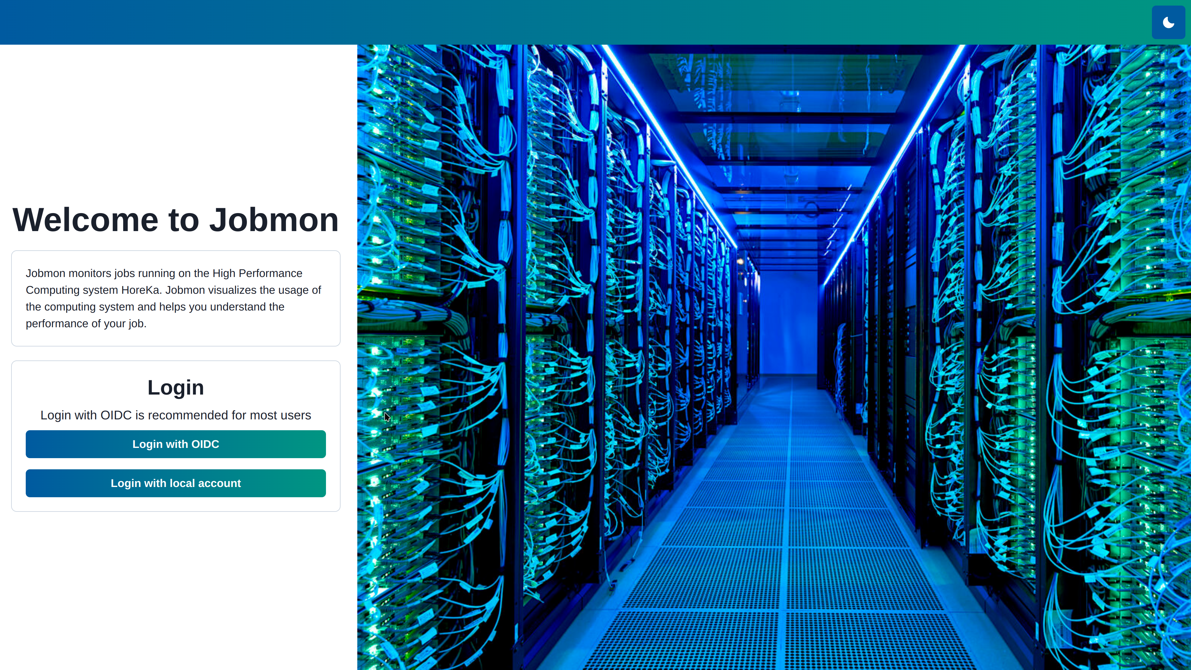
Log in via:
- FeLS authentication
- Local account
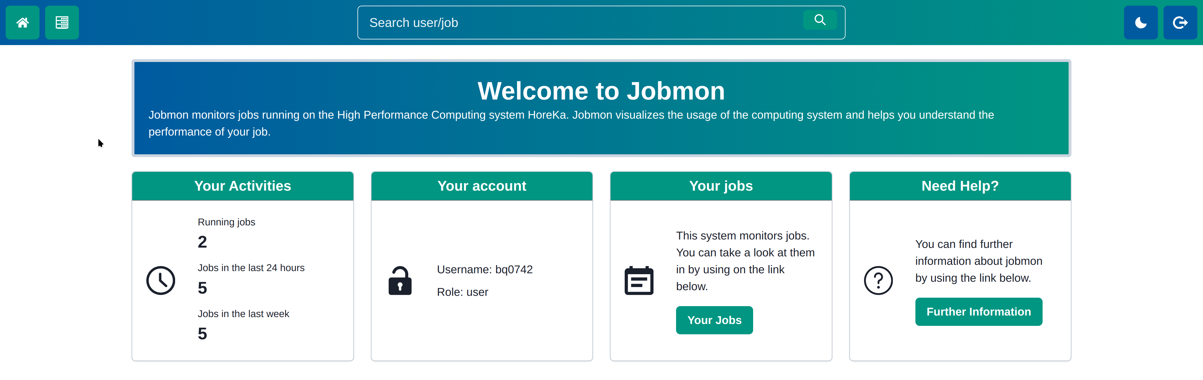
You will typically find:
- User information
- Job statistics: number of jobs in the last week, number of finished jobs, number of running jobs
Data retention policy
Metrics are retained for 90 days. Job metadata is retained for longer, but time-series diagrams no longer contain metric data for jobs older than 90 days.
Privacy model
Users can only view metrics for their own jobs. Administrators have additional privileges (e.g., viewing all jobs, applying system-wide tags, viewing system-wide metrics and statistics).
Sharing jobs with external users
Jobs can also be shared with people who do not have a cluster account. The job owner or an administrator can enable the guest view and generate a unique link that provides read-only access to the job.
Analyzing jobs
Job performance commonly falls into one (or more) of the following categories:
- Compute bound: CPU/GPU compute throughput is the limiting factor.
- Memory bound: Memory bandwidth or latency is the limiting factor.
- Communication bound: Node-to-node communication is the limiting factor.
- I/O bound: Filesystem throughput or metadata performance is the limiting factor.
Jobs are often mixed
Many real workloads alternate between phases (e.g., compute → communication → I/O checkpoint). Use the per-job time series to isolate the steady-state region of each phase.
Interpret metrics together
Individual metrics usually provide indicators rather than definitive proof of a bottleneck. Correlate compute, memory, communication, and I/O metrics over the same time range before drawing conclusions about the limiting resource.
What to look for in JobMon
Compute bound
-
Typical signals: sustained CPU FLOP/s and/or GPU utilization together with comparatively lower pressure on memory, communication, and I/O resources.
-
Where to investigate: Performance (FLOP/s, IPC, GPU utilization), then correlate with Memory, Interconnect, and Filesystem as needed.
CPU FLOP/s and floating-point precision
JobMon currently measures CPU floating-point activity only for 64-bit floating-point operations. Workloads that primarily use 32-bit floating-point arithmetic may therefore show very low FLOP/s values or no FLOP/s data, even when they are compute-intensive.
A low CPU FLOP/s value should therefore not, by itself, be interpreted as evidence that a job is not compute-bound.
Memory bound
- Typical signals: sustained CPU memory bandwidth with comparatively low compute throughput; on GPUs, sustained memory activity together with lower compute utilization than expected for the workload.
- Where to investigate: Memory (CPU bandwidth, GPU memory utilization), then correlate with Performance (IPC/FLOP/s).
Communication bound
- Typical signals: sustained or phase-correlated InfiniBand traffic and/or packet rates, often accompanied by reduced CPU/GPU activity while communication dominates.
- Where to investigate: Interconnect (send/receive bandwidth and packet rates), then correlate with Performance.
I/O bound
- Typical signals: sustained filesystem throughput, high metadata-operation rates, or periodic bursts associated with checkpointing. CPU/GPU utilization may decrease during these phases.
- Where to investigate: Filesystem (throughput, IOPS, and metadata operations), correlated with Performance.
To illustrate these patterns, the next sections use representative benchmarks.
Compute bound
Performance is limited by CPU and/or GPU compute throughput (typically floating-point operations). Benchmarks from this category include:
-
DGEMM performs a matrix–matrix multiplication
C = A · B. Forn×nmatrices, it requiresO(n^3)compute operations but onlyO(n^2)memory operations. CPU and GPU implementations exist.Characteristics
- High CPU FLOP/s (CPU run) or high GPU utilization (GPU run)
- Moderate CPU memory bandwidth usage compared to compute saturation
Memory bound
Performance is limited by the main memory subsystem (bandwidth and/or latency). Benchmarks from this category include:
-
STREAM performs four kernels: copy (
c=a), scale (b=α·c), add (c=a+b), and triad (a=b+α·c). It stresses memory bandwidth heavily. For n-dimensional vectors, computation requiresO(n)memory operations but onlyO(n)compute operations. CPU and GPU implementations are available for this benchmark.Characteristics
- CPU memory bandwidth near peak (CPU STREAM)
- GPU memory utilization near saturation (BabelStream on GPU)
- Compute metrics (FLOP/s, IPC) typically very low.
-
High Performance Conjugate Gradients (HPCG)
HPCG runs conjugate gradients on a sparse matrix and is commonly used as a proxy for memory-bound, irregular access patterns. CPU and GPU implementations exist.
Characteristics
- Sustained memory pressure over time
- Often clear phase behavior (setup vs solve), depending on implementation
Communication bound
Performance is limited by the interconnect (bandwidth and/or latency). Benchmarks from this category include:
-
OMB performs point-to-point communication with messages of increasing size to measure bandwidth and latency (CPU and GPU variants exist).
Characteristics
- InfiniBand send/receive bandwidth and packet rates rising with message size
- Visible "steps" when the message size changes
I/O bound
Performance is limited by filesystem throughput and/or metadata operations. These cases are common in checkpointing, heavy file-per-rank workloads, and metadata-intensive pipelines.
Benchmarks from this category include:
-
Characteristics
- IOR: sustained or bursty read/write throughput; periodic spikes are typical for checkpoint patterns
Jobs page
This page presents an overview of your recent batch jobs on JobMon. Jobs can be filtered by:
- partition
- exit codes
- number of nodes / number of GPUs
- job status (finished/running/all)
- time range (e.g., last week)
- tags (e.g.,
baseline,optA,optB)
The filtered jobs can be sorted by:
- job length
- number of nodes
- start time
- stop time
- job ID

Each job displayed on the Jobs page is represented by its metadata and a spider plot. The spider plot provides a high-level summary of resource utilization and can help identify whether a job is worth investigating as compute-, memory-, or communication-intensive. It should be treated as an indicator rather than a definitive bottleneck classification, particularly for jobs with multiple execution phases.
CPU compute activity may also be underestimated for applications that primarily use 32-bit floating-point arithmetic, because the CPU FLOP/s metric currently covers only 64-bit floating-point operations.
- CPU floating-point operations per second (FLOP/s)
- CPU memory bandwidth
- GPU utilization
- GPU memory utilization
- InfiniBand bandwidth
Examples: Spider Plot
.png)
DGEMM is capable of using the entire available floating-point power of the node. This also uses a significant portion of the memory bandwidth.
.png)
STREAM saturates the entire memory bandwidth. All other resources are under-utilized.
.png)
OSU Micro-Benchmarks saturates the entire InfiniBand bandwidth. Some memory bandwidth utilization can also be seen as messages are transferred from memory to memory.
.png)
The DGEMM implementation uses only a single GPU. Therefore, only a quarter of the available floating-point performance of the GPUs is utilized. This is reflected in the use of memory bandwidth as well.
.png)
HPCG runs distributed on all GPUs of the node. HPCG saturates the entire memory bandwidth of these GPUs. The compute units are also well utilized.
.png)
InfiniBand communication between GPUs is not as performant as between CPUs. Therefore, OSU Micro-Benchmarks cannot utilize the entire available InfiniBand bandwidth.
Spider plot
The spider plot depends on the availability and successful analysis of the underlying metrics. If metrics are missing or analysis fails, the plot may be empty or contain missing axes. Always inspect the per-job time series before drawing conclusions from the spider plot alone.
Per-job page
Configuration options
- Node filtering: Show only nodes of interest.
- Metric filtering: Show only selected metrics.
- Time range selection: Restrict all diagrams to a specific time range using the range slider.
-
Tag modification:
Tags are a handy tool to mark jobs during different optimization steps (e.g. tags: "without optimization", "optimization A", "optimization B", ...) or jobs from different workflows (e.g. tags: "workflow A", "workflow B"). Filtering for tags on the jobs page allows easily finding all jobs with the same tag.
-
Set sample rate:
Different sampling intervals are available, particularly for longer jobs. Smaller intervals provide more detail but require more data to be retrieved and rendered.
-
Toggle for Automatic Scaling:
Automatically determine diagram y-axis limits from the displayed values.
-
Toggle for Changepoints:
Changepoint detection identifies candidate times at which metric behavior changes. Detected changepoints are displayed as vertical lines in the diagrams. They are indicators of behavioral changes and do not necessarily correspond to application-phase boundaries.
-
Toggle for Quantile view:
- Quantile view is a useful feature to improve clarity when too many graphs are displayed in one diagram.
- The displayed series are condensed into the 25th, 50th, and 75th percentiles.
- At each timestamp, the 25th percentile indicates the value below which 25% of the displayed measurements fall.
- The 50th percentile is also known as the median.
- The interval between the 25th and 75th percentiles is the interquartile range and provides an indication of the spread between the displayed series.
Examples: Quantile View
.png)
The CPU temperatures are collected per hardware thread; therefore, the diagram appears very cluttered.
.png)
The Quantile View shows the distribution of CPU temperatures more clearly.
.png)
The CPU frequencies are collected per CPU core; therefore, the diagram appears very cluttered.
.png)
The Quantile View shows the distribution of CPU frequencies more clearly.
Performance categories
Metrics are grouped into the following categories.
Energy
This category offers diagrams for:
- CPU power consumption of DRAM channels and the package
- GPU power consumption
- Server system power consumption
Examples: Category Energy
.png)
STREAM, as a memory-bound benchmark, puts constant pressure on the DRAM subsystem. This is reflected by the consistently high power consumption of this subsystem.
.png)
DGEMM, as a compute-bound benchmark, puts less pressure on the DRAM subsystem. This is reflected in the varying power consumption of the DRAM subsystem over time.
.png)
The GPU implementation of the HPCG benchmark has a preparation phase executed on the CPU and a computation phase executed on the GPU. During the first phase, the power consumption of the CPU package is therefore higher than in the subsequent phase.
.png)
The GPU implementation of the HPCG benchmark has a preparation phase executed on the CPU and a computation phase executed on the GPU. During the first phase, the power consumption of the GPUs is therefore lower than in the subsequent phase.
Filesystem
This category offers the following diagrams for Home and Workspace filesystems:
- I/O operations/s (reads and writes)
- Read/write throughput (bytes/s)
- Metadata operations/s
Examples: Category Filesystem
.png)
Bytes read for the IOR benchmark.
.png)
Bytes written for the IOR benchmark.
.png)
Total throughput for the IOR benchmark.
Interconnect
This category offers diagrams for:
- InfiniBand: Send, receive and aggregated bandwidth
- InfiniBand: Send, receive and aggregated number of packets
Examples: Category Interconnect
.png)
InfiniBand send bandwidth for OSU Micro-Benchmark. In the point-to-point communication, node hkn0201 sends data while node hkn0202 only receives data (send bandwidth is zero).
.png)
InfiniBand receive bandwidth for OSU Micro-Benchmark. In the point-to-point communication, node hkn0202 receives data while node hkn0201 only sends data (receive bandwidth is zero).
.png)
InfiniBand bandwidth for OSU Micro-Benchmark. In the point-to-point communication, both nodes use the same bandwidth, even though one of the nodes only sends data and the other one only receives data.
Memory
This category offers diagrams for:
- Amount of memory used on the system (CPU) and on the GPU
- CPU memory bandwidth
- GPU memory utilization (in %) and frequency
Examples: Category Memory
.png)
STREAM, as a memory-bound benchmark, puts constant pressure on the memory subsystem.
.png)
DGEMM, as a compute-bound benchmark, puts less pressure on the memory subsystem. This is reflected in the varying bandwidth over time.
.png)
Babelstream, as a memory-bound benchmark, fully utilizes the memory subsystem of the GPU.
.png)
The GPU implementation of DGEMM, as a compute-bound benchmark, puts less pressure on the GPU memory subsystem. This is reflected in the varying utilization over time.
Performance
This category offers diagrams for:
- 64-bit floating-point operations per second (FLOP/s), collected per hardware thread and aggregated per core or per socket
Note
CPU FLOP/s currently covers only 64-bit floating-point operations. Applications that predominantly use 32-bit floating-point arithmetic may therefore report very low FLOP/s values or no FLOP/s data.
- Instructions per cycle (IPC), collected per hardware thread and aggregated per core or per socket
- CPU time spent in kernel and in user space
- One-minute Linux load average
- GPU utilization
- CPU and GPU frequencies
Examples: Category Performance
.png)
FLOP/s are collected per hardware thread. Because hardware threads on the same core share execution resources, aggregation per core can make core-level utilization easier to interpret.
.png)
FLOP/s are collected per hardware thread. Aggregation per socket can be useful for comparing utilization across CPU sockets.
Temperature
This category offers diagrams for:
- CPU and GPU temperatures
Examples: Category Temperature
.png)
The GPU implementation of the DGEMM benchmark only utilizes one of the GPUs. Only this GPU gets hot, while the other GPUs maintain a lower temperature.
.png)
The GPU implementation of the HPCG benchmark has a preparation phase executed on the CPU and a computation phase executed on the GPU. During the first phase, the GPU is not utilized and therefore stays cooler than in the subsequent phase.
Additional Features
- For multi-node jobs, there is a configuration option to select the per-node aggregation function used (e.g., average, sum, maximum).
- Running jobs provide a live view covering the most recent 10 minutes.
- Export metrics for offline analysis.
- Favorite metric category
- The default category is Performance. You can change it using the star button.
- Metric analyzers:
- Changepoint analyzer: A heuristic analyzer that marks times where metric behavior changes.
- I/O analyzer: Analyzes I/O metrics by comparing the mean rate and the final sum against predefined threshold values. If thresholds are exceeded, tags are applied.
- Roofline chart: Relates achieved floating-point performance to arithmetic intensity and can help distinguish workloads constrained primarily by memory bandwidth from those approaching a compute-performance limit.
- Job sharing: Use the Share button to create a unique link through which other users can inspect the job in read-only mode.
Changepoint metrics
To avoid excessive load on the time-series database, changepoints are computed only for a subset of metrics selected by administrators. The sample rate at which they are computed is also chosen automatically.
Performance tips
-
Filter out metrics that are not relevant to your analysis. This can significantly improve readability and loading time in categories containing many metrics.
-
Choose a favorite category so that JobMon initially loads the metrics most relevant to your workflow.
-
JobMon selects a sample rate automatically. Selecting a very small sampling interval increases the amount of data retrieved and can substantially increase loading time.